Logistic Regression in Python

Logistic regression is the most basic algorithm for classfication. It extends the idea of linear regression to cases where the dependent variable only has a discrete number of outcomes, which are also called classes. Depending on the number of possible outcomes, we can classify logistic regression models into two types: binary logistic regression and multiple logistic regression.

Instead of modeling Y as a linear function of X directly, we model the probability that is equal to class 1, given X.

For this tutorial, we are going to use logistic regression to predict whether a patient has 10-year-risk of future coronary heart disease. The dataset can be downloaded here.

We can import all the required libraries and our dataset:

import pandas as pd
import numpy as np
import matplotlib.pyplot as plt
import statsmodels.api as sm
from sklearn.model_selection import train_test_split
from sklearn.linear_model import LinearRegression
from sklearn.metrics import classification_report
from sklearn.metrics import confusion_matrix
from sklearn.metrics import accuracy_score
from statsmodels.tools import add_constant as add_constant

grad_admissions = pd.readcsv('/Users/mengjialyu/Documents/Kaggle/graduate-admissions/Admission_Predict.csv')

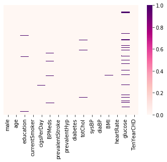
Data preprocessing is an important initial step when doing machine learning projects. seaborn is a great library that can provide a visualization of missing data. The cmap here refers to the mapping from data values to color space, and RdPu is one color scheme option among many available. An alternative method is to simply display the sum of missings value in each data columnm.

sns.heatmap(heart_disease.isnull(), yticklabels = False, cmap = 'RdPu')

# another way to check null values
heart_disease.isnull.sum()

Now we have this pretty little graph :)

It looks like do not have much missing data. So we can exclude the rows with missing values.

heart_disease.dropna(axis = 0, inplace = True)

Let’s move on and fit a logistic regression model to our data. First we need to filter out the features that really matters.

heart_add_const = add_constant(heart_disease)
cols=heart_df.columns[:-1]

def back_feature_elem (data_frame,dep_var,col_list):
    while len(col_list)>0 :
        model=sm.Logit(dep_var,data_frame[col_list])
        result=model.fit(disp=0)
        largest_pvalue=round(result.pvalues,3).nlargest(1)
        if largest_pvalue[0]<(0.05):
            return result
            break
        else:
            col_list=col_list.drop(largest_pvalue.index)

result=back_feature_elem(heart_add_const,heart_disease.TenYearCHD,cols)
print(result.params)

const -9.129843 male 0.561446 age 0.065896 cigsPerDay 0.019226 totChol 0.002272 sysBP 0.017534 glucose 0.007280

The results show that const, male, age, cigsPerDay, totChol, sysBP, glucose are features that matter! From the data-description, we know that male is a nominal variable. To apply a egression analysis on any dataset, normally we have to first tranform categorical features to dummy variables using the get_dummies() function from pandas. Dummy variables assign numerical values to the original categorical levels so that the computers can compute on them :) (More about one-hot encoding)

However for categorical variable with only two levels, there is no need to create dummy variables. As sex is binary in our dataset, we can leave it as it is.

X_train, X_test, y_train, y_test = train_test_split(X, y, test_size=0.2, random_state=0)

log_regressor = LogisticRegression()
log_regressor.fit(X_train, y_train)

y_pred = log_regressor.predict(X_test)

how acccurate is our model?

print(classification_report(y_test, y_pred))

print(confusion_matrix(y_test, y_pred))


accuracy_score(y_test,y_pred)

The accuracy turns out to be 85.5%. Good enough ;)

References:

Advanced Methods for Data Analysis Course Note

Notes Andrew NG Course

Medium Post

Kaggle Notebook