AI Markov Decision Process
Markov Processes
Introduction to MDPs
- Markov decision process formally describe an environment for reinforcement learning
- Where the environment is fully observable
- i.e. The current state completely characterizes the process
- Almost all RL problems can be formalized as MDPs
- Optimal control primarily deals with continuous MDPs
- Partially observable problems can be converted into MDPs
- Bandits are MDPs with one state
Markov Property
“The future is independent of the past given the present”
-
The state captures all relevant information from the history.
- Once the state is known, the history may be thrown away
- i.e. The state is a sufficient statistic of the future.
State Transition Matrix
For a Markov state s and successor state $s’$, the state transition probability is defined by:
\[\mathcal{P} = P[S_{t+1}=s' | S_t=s]\]State transition matrix $\mathcal{P}$ defines transition probabilities to all successor states $s’$
\(\mathcal{P} = \begin{bmatrix} \mathcal{P}_{11} & \cdots & \mathcal{P}_{11} \\ \vdots \\ \mathcal{P}_{11} & \cdots & \mathcal{P}_{nn} \end{bmatrix}\) where each row of the matrix sums to 1.
Markov Process
A Markov process is a memoryless random process, i.e. a sequence of random states $S_1$, $S_2$, $\cdots$ with the Markov property.
Markov Reward Processes
Markov Reward Process
A Markov reward process is a Markov chain with values.
- $\gamma$ is the discount factor
Return
- The discount $\gamma$ is the present value of future rewards
- The value of receiving R after k+1 time-steps is ${\gamma}^k R$
- This values immediate reward above delayed reward
- $\gamma$ close to 0 leads to “myopic” evaluations
- $\gamma$ close to 1 leads to “far-sighted” evaluation
Why discount?
Most Markov reward and decision processes are discounted.
- Mathematically convenient to discount rewards
- Avoids infinite returns in cyclic Markov processes
- Uncertainty about the future may not be fully represented
- If the reward is financial, immediate rewards may earn more interest than delayed rewards
- Animal/human behavior shows preference for immediate reward
- It is sometimes possible to use undiscounted Markov reward processes (i.e. $\gamma=1$), e.g. if all sequences terminate
Value Function
- The value function $v(s)$ gives the long-term value of state s
Bellman Equation for MRPs
The value function can be decomposed into two parts:
- immediate reward R_{t+1}
- discounted value of successor state $\gamma v(S_{t+1})$
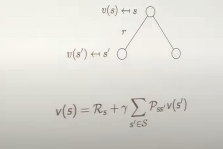
Bellman Equation in Matrix Form
The Bellman equation can be expressed concisely using matrices,
\(v = \mathcal{R} + \gamma \mathcal{P}v\) where v is a column vector with one entry per state
\[\begin{bmatrix} v_{1} \\ \vdots \\ v_{n} \end{bmatrix} = \begin{bmatrix} \mathcal{R}_{1} \\ \vdots \\ \mathcal{R}_{n} \end{bmatrix} + \gamma\begin{bmatrix} \mathcal{P}_{11} & \dots & \mathcal{P}_{1n} \\ \vdots \\ \mathcal{P}_{11} & \dots & \mathcal{P}_{nn} \end{bmatrix}\begin{bmatrix} v_{1} \\ \vdots \\ v_{n} \end{bmatrix}\]$R_n$ represents the reward enjoyed for exiting state n.
Solving the Bellman Equation
- The Bellman equation is a linear equation
- It can be solved directly $$ v = \mathcal{R} + \gamma \mathcal{R} v
(I - \gamma \mathcal{R})v = \mathcal{R}
v = (I - \gamma \mathcal{R})^{-1}\mathcal{R} $$
- Computational complexity (matrix inversion) $O(n^3)$ for n states
- Direct solution only possible for small MRPs
- There are many iterative methods for large MRPs
- Dynamic programming
- Monte-Carlo evaluation
- Temporal-Difference learning
Markov Decision Processes
Markov Decision Process
Policies
- A policy fully defines the behavior of an agent
- MDP policies depend on the current state (not the history)
- i.e., Policies are stationary (time-independent), $A_t ~ \pi(\dot | S_t)
- Given an MDP $\mathcal{M}=\langle \mathcal{S},\mathcal{A}, \mathcal{P}, \mathcal{R}, \gamma \rangle$ and a policy $\pi$
- The state sequence $S_1, S_2, \dots$ is a Markov process \langle \mathcal{S},\mathcal{P}_{\pi} \rangle
- The sate and reward sequence, $S_1, R_2, S_2, \dots$ is a Markov Reward process $S, \mathcal{P}{\pi} , \mathcal{R}{\pi} , \gamma$
Value Function
E.g. action: take left or right?
Bellman Expectation Equation
The state-value function can again be decomposed into immediate reward plus discounted value of successor state.
\[v_\pi(s) = E_\pi [R_{t+1} +\gamma v_\pi(S_{t+1}) | S_t = s]\]The action-value function can similarly be decomposed,
\[q_\pi(s,a) = E_\pi [R_{t+1} +\gamma q_\pi(S_{t+1}, A_{t+1}) | S_t = s, A_t = a]\]Bellman Expectation Equation for $v_\pi$
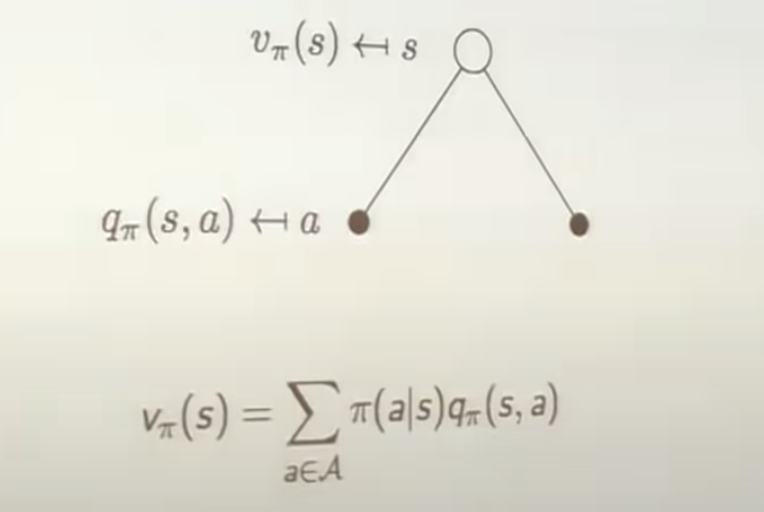
Bellman Expectation Equation for $q_\pi$
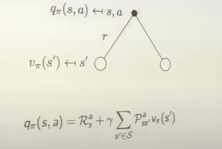
Bellman Expectation Equation for $v_\pi$ - revisit
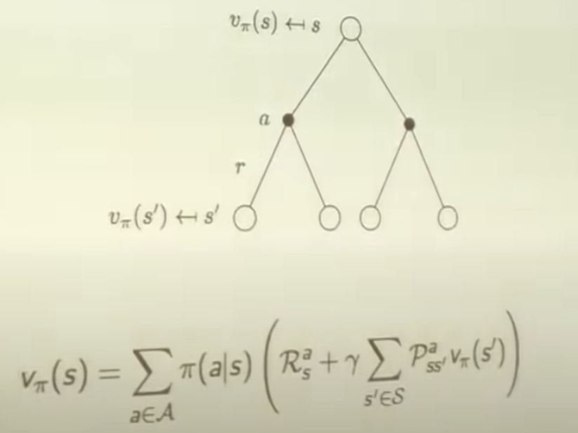
How to find the best decison?
Bellman Expectation Equation (Matrix Form)
The Bellman expectation equation can be expressed concisely using the induced MRP, \(v_\pi = \mathcal{R}^{\pi} + \gamma \mathcalP^{\pi}v_\pi\) Direct solution is \(v_\pi = (I - \gamma \mathcal{P}^{\pi})^{-1} \mathcalR^{\pi}\)
Optimal Value Function
-
THe optimal value function specifies the best possible performance in MDP.
-
An MDP is “solved” when we know the optimal value fn/finding q*.
Optimal Policy
Define a partial ordering over policies \(\pi \geq \pi' if v_\pi (s) \geq v_{\pi'}(s) \forall s\)
Finding an Optimal Policy
An optimal policy can be found by maximizing over $q_* (s,a)$
- There is always a deterministic optimal policy for any MDP
- If we know $q_* (s,a)$, we immediately have the optimal policy
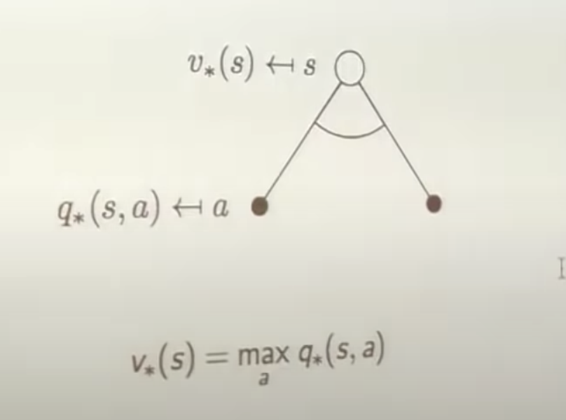
Bellman Optimality Equation for $v_*$
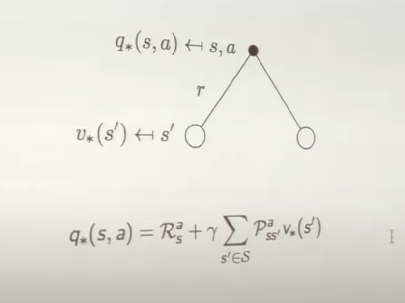
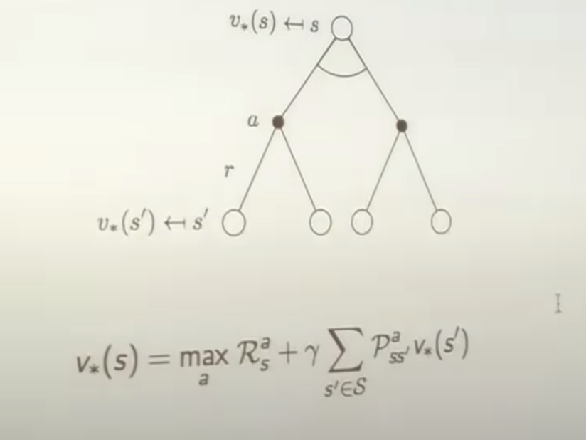
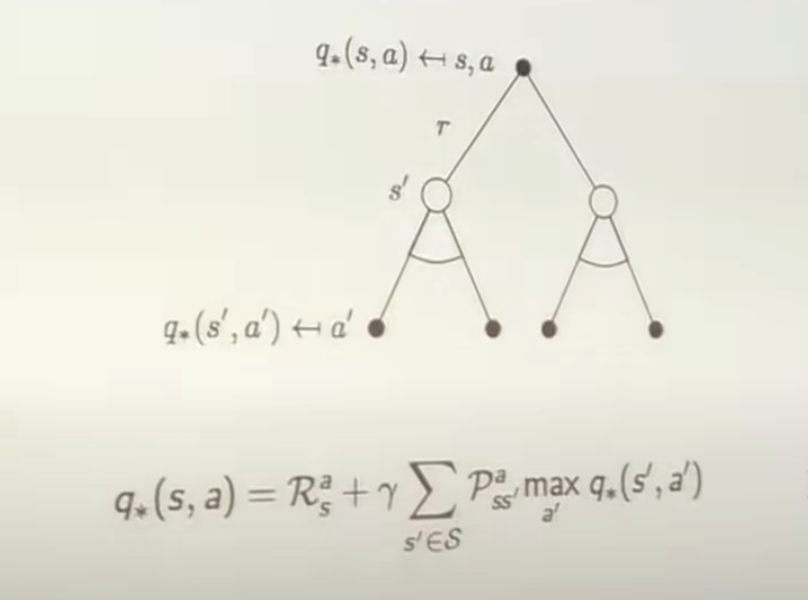
The optimal value functions as recursively related by the Bellman optimality equations:
\(v_* (s) = \max_a q_*(s,a)\)
Bellman Optimality Equation for $q_*$
Bellman Optimality Equation for $v_*$ - revisit
Bellman Optimality Equation for $q_*$ - revisit
Solving the Bellman Optimality Equation
- Bellman Optimality Equation is non-linear
- No closed form solution (in general)
- Many iterative solution methods
- Value Iteration
- Policy Iteration
- Q-learning
- Sarsa
Approaches to uncertainty:
- Explicitly represent in MDP
- Factor in uncertainty in MDP itself
- Sufficient to make discount factor
Bellman’s principle of optimality
The dynamic programming method breaks this decision problem into smaller subproblems. Bellman’s principle of optimality describes how to do this:
Principle of Optimality: An optimal policy has the property that whatever the initial state and initial decision are, the remaining decisions must constitute an optimal policy with regard to the state resulting from the first decision. (See Bellman, 1957, Chap. III.3.)[Wikipedia]
Extensions to MDPs
- Infinite and continuous MDPs
- Partially observable MDPs
- Undiscounted, average reward MDPs