Introduction

Estimate the value function of an unknown MDP

Monte-Carlo Reinforcement Learning

MC methods learn directly from episodes of experience
MC is model-free
- No knowledge of MDP transitions/rewards
MC learns from complete episodes: no bootstrapping
MC uses the simplest possible idea
- value = mean return
Caveat
- Can only apply MC to episodic MDPs
- All episodes must terminate

Monte-Carlo Policy Evaluation

Goal: learn $v_\pi$ from episodes of experience under policy $\pi$
Return is the total discounted reward:

\[G_t = R_{t+1} + \gamma R_{t+2} + \dots + \gamma^{T-1} R_T\]

Value function is the expected return: $v_\pi(s) = R_{\pi} [G_t | S_t = s]$
Monte-Carlo policy evaluation uses empirical mean return instead of expected return

First-Visit Monte-Carlo Policy Evaluation

To evaluate state s
- The first time-step t that state s is visited in an episode
- increment counter $N(s) += 1$
- increment total return $S(s) = S(s) + G_t$
- value is estimated by mean return $V(s) = \frac{S(s)}{N(s)}
- by law of large numbers, $V(s) = v_pi(s) as N(s) approaches infinity.

Every-visit Monte-Carlo Policy Evaluation

To evaluate state s
- Every time-step t that state s is visited in an episode,
- increment counter $ N(s) += 1$
- increment total return $S(s) = S(s) + G_t$
- value is estimated by mean return $V(s) = \frac{S(s)}{N(s)}
- by law of large numbers, $V(s) = v_pi(s) as N(s) approaches infinity.

Incremental Mean

The mean $\mu_1, \mu_2, \dots$ of a sequence can be computed incrementally

\[\mu_k = \frac{\sum_{j=1}^k x_j}{k}\] \[\mu_k = \mu_{k-1} + \frac{x_k -\mu_{k-1}}{k}\]

Incremental Monte-Carlo Updates

Update V(s) incrementally after episodes $S_1,A_1,$
- For each state $S_t$ with return $G_t$ $$ N(S_t) = N(S_t) + 1
V(S_t) = V(S_t) + \frac{G_t - V(S_t)}{N(S_t)} $$
In non-stationary problems, it can be useful to track a running mean, i,e, forget old episodes. $$

V(S_t) = V(S_t) + \alpha (G_t - V(S_t)) $$

Temporal-Difference Learning

TD methods learn directly from episodes of experience
TD is model-free: no knowledge of MDP transitions/rewards
TD learns from incomplete episodes, by bootstrapping
TD updates a guess towards a guess

MC and TD

Goal: learn $v_\pi$ online from experience under policy $\pi$
Incremental every-visit Monte-Carlo
- Update value $V(S_t)$ toward actual return $G_t$
Simplest temporal-difference learning algorithm: TD(0)
- Update value $V(S_t)$ toward estimated return $$
V(S_t) = V(S_t) + \alpha (R_{t+1} + \gamma V(S_{t+1}) - V(S_t))$ $$
- $R_{t+1} + \gamma V(S_{t+1})$ is called the TD target
- $\delta_t = R_{t+1} + \gamma V(S_{t+1}) - V(S_t)$ is called the TD error

Pros and Cons of MC vs TD

TD can learn before knowing the final outcome
- TD can learn online after every step
  - MC must wait until end of episode before return is known
TD can learn without the final outcome
- TD can learn from incomplete sequences
  - MC can only learn from complete sequences
- TD works in non-terminating environments
  - MC only works for episodic/terminating environments
MC has high variance, zero bias
- Good convergence properties even with function approximation
- Not very sensitive to initial value
- Very simple to understand and use
TD has low variance, some bias
- Usually more efficient than MC
- $TD(0)$ converges to $v_pi(s)$, but not always with function approximation
- More sensitive to initial value
TD expoits Markov property
- Usually more efficient in Markov environments
MC does not exploit Markov property
- Usually more effective in non-Markov environments

Bootstrapping and Sampling

Bootstrapping: update involves an estimate
- MC does not bootstrap
- DP bootstraps
- TD bootstraps
Sampling: update samples an expectation
- MC samples
- DP does not sample
- TD samples

TD($\lambda$)

n-step Prediction

Let TD target look n steps into the future
Define the n-step return
n-step temporal-difference learning

Large Random Walk Example

Averaging n-step Returns

We can average n-step returns over different n
e.g. average the 2-step and 4-step returns
Combines information from two different time-steps
Can we efficiently combine information from all time-steps?

$\lambda$-return

$TD(\lambda)$ Weighting Function

Forward-view $TD(\lambda)$

Update value function towards the $TD(\lambda)$
Forward-view looks into the future to compute $G_t^{\lambda}$
Like MC, can only be computed from complete episodes

Forward-view $TD(\lambda)$ on Large Random Walk

Backward View $TD(\lambda)$

Forward view provides theory
Backward view provides mechanism
Update online, every step, from incomplete sequences

Eligibility Traces

Credit assignment problem: did bell or light cause shock?
Frequency heuristic: assign credit to most frequent states
Recency heuristic: assign credit to most recent states
Eligibility traces combine both heuristics

Backward View $TD(\lambda)$

Keep an eligibility trace for every state s
Update value V(s) for every state s
In proportion to TD-error and eligibility trace

$TD(\lambda)$ and $TD(0)$

when $\lambda$ = 0 , current state is updated

$TD(\lambda)$ and MC

When $\lambda$ = 0, credit is deferred until end of episode
Consider episodic environments with offline updates
Over the course of an episode, total update for $\lambda$ = 0 is the same as total update for MC

$TD(1)$ and MC

Consider an episode where s is visited once at time-step k

Telescoping in $TD(\lambda)$

$TD(\lambda)$ and $TD(1)$

Telescoping in $TD(\lambda)$

Forwards and Backwards in $TD(\lambda)$

$TD(\lambda)$ eligibility trace discounts time since visit

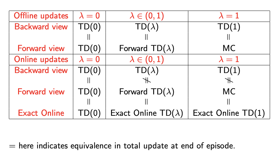
Offline Equivalence of Forward and Backward TD

Offline updates are accumulated within episode
- applied in batch at the end of the episode

Online Equivalence of Forward and Backward TD

$TD(\lambda)$ updates are applied online at each step within episode
Forward and backward-view $TD(\lambda)$ are slightly different
Exact online $TD(\lambda)$ achieves perfect equivalence
By using a slightly different form of eligibility trace

Final Summary

backpropagation